from sklearn.linear_model import Perceptron
import numpy as np
import matplotlib.pyplot as plt인공신경망과 퍼셉트론
인공신경망
퍼셉트론
ref
기본 원리
- AND/OR/XOR연산
| 표본 | \(x_1\) | \(x_2\) | \(x_1 AND x_2\) | \(x_1 OR x_2\) | \(x_1 XOR x_2\) |
|---|---|---|---|---|---|
| 1 | 0 | 0 | 0 | 0 | 0 |
| 2 | 1 | 0 | 0 | 1 | 1 |
| 3 | 0 | 1 | 0 | 1 | 1 |
| 4 | 1 | 1 | 1 | 1 | 0 |
1. 패키지 설정
2. 데이터 준비
# 데이터 작성(OR연산)

X=np.array([[0,0],[0,1],[1,0],[1,1]])
y=np.array([0,1,1,1])
3. 탐색적 데이터 분석
plt.scatter(X[:,0], X[:,1], c=y)
plt.xlabel('x1')
plt.ylabel('x2')
plt.show()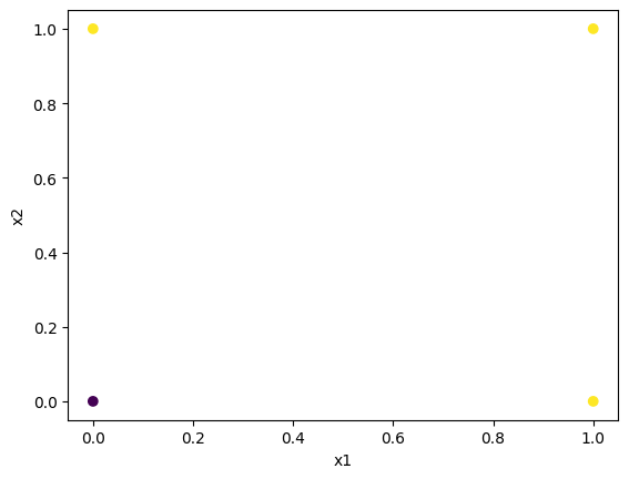
4. 모형화 및 학습
model=Perceptron(verbose=1)
model.fit(X,y)
-- Epoch 1
Norm: 1.41, NNZs: 2, Bias: 0.000000, T: 4, Avg. loss: 0.250000
Total training time: 0.00 seconds.
-- Epoch 2
Norm: 2.24, NNZs: 2, Bias: 0.000000, T: 8, Avg. loss: 0.000000
Total training time: 0.00 seconds.
-- Epoch 3
Norm: 2.24, NNZs: 2, Bias: -1.000000, T: 12, Avg. loss: 0.000000
Total training time: 0.00 seconds.
-- Epoch 4
Norm: 2.83, NNZs: 2, Bias: 0.000000, T: 16, Avg. loss: 0.000000
Total training time: 0.00 seconds.
-- Epoch 5
Norm: 2.83, NNZs: 2, Bias: -1.000000, T: 20, Avg. loss: 0.000000
Total training time: 0.00 seconds.
-- Epoch 6
Norm: 2.83, NNZs: 2, Bias: -1.000000, T: 24, Avg. loss: 0.000000
Total training time: 0.00 seconds.
-- Epoch 7
Norm: 2.83, NNZs: 2, Bias: -1.000000, T: 28, Avg. loss: 0.000000
Total training time: 0.00 seconds.
Convergence after 7 epochs took 0.00 secondsPerceptron(verbose=1)In a Jupyter environment, please rerun this cell to show the HTML representation or trust the notebook.
On GitHub, the HTML representation is unable to render, please try loading this page with nbviewer.org.
Perceptron(verbose=1)
학습계수 eta0=1
학습 종료 기준 허용오차 0.001
이전 단계 epoch의 평균 비용과 현재 epoch의 평균 비용과의 차이가 허용오차보다 작으면 학습 종료ㅡ
# 가중치
print(model.coef_)
# 편향
print(model.intercept_)
# 학습 수(epoch)
print(model.n_iter_)
[[2. 2.]]
[-1.]
7\[x_2=\dfrac{w_1}{w_2}x_1 - \dfrac{b}{w_2}\]
\[x_2=-\dfrac{2}{2}x_1 - \dfrac{-1}{2}= -x_1+\dfrac{1}{2}\]
#산포도
plt.scatter(X[:,0], X[:,1],c=y)
plt.xlabel('x1')
plt.ylabel('x2')

#파라미터
w1=model.coef_[0,0]
w2=model.coef_[0,1]
b=model.intercept_

#x절편
x_intercept=-b/w1
#y절편
y_intercept=-b/w2
#선형 분류자 추가
plt.plot([0,y_intercept],[x_intercept,0], c='red')
plt.show()
/home/coco/anaconda3/envs/py38/lib/python3.8/site-packages/numpy/core/shape_base.py:65: VisibleDeprecationWarning: Creating an ndarray from ragged nested sequences (which is a list-or-tuple of lists-or-tuples-or ndarrays with different lengths or shapes) is deprecated. If you meant to do this, you must specify 'dtype=object' when creating the ndarray.
ary = asanyarray(ary)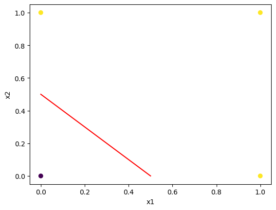
5. 예측
X_test=X
pred=model.predict(X_test)
print(pred)
[0 1 1 1]붗꽃 분류
- 4개의 입력 노드와 1개의 출력 노드로 구성
1. 패키지 설정
from sklearn import datasets
from sklearn.preprocessing import StandardScaler
from sklearn.linear_model import Perceptron
from sklearn.model_selection import train_test_split
from sklearn.metrics import accuracy_score
import numpy as np
import matplotlib.pyplot as plt
import pandas as pd
import seaborn as sns
2. 데이터 준비
iris = datasets.load_iris()
print(iris.feature_names)
print(iris.target_names)
['sepal length (cm)', 'sepal width (cm)', 'petal length (cm)', 'petal width (cm)']
['setosa' 'versicolor' 'virginica']X=iris.data
y=iris.target
print(X[:10])
print(y)[[5.1 3.5 1.4 0.2]
[4.9 3. 1.4 0.2]
[4.7 3.2 1.3 0.2]
[4.6 3.1 1.5 0.2]
[5. 3.6 1.4 0.2]
[5.4 3.9 1.7 0.4]
[4.6 3.4 1.4 0.3]
[5. 3.4 1.5 0.2]
[4.4 2.9 1.4 0.2]
[4.9 3.1 1.5 0.1]]
[0 0 0 0 0 0 0 0 0 0 0 0 0 0 0 0 0 0 0 0 0 0 0 0 0 0 0 0 0 0 0 0 0 0 0 0 0
0 0 0 0 0 0 0 0 0 0 0 0 0 1 1 1 1 1 1 1 1 1 1 1 1 1 1 1 1 1 1 1 1 1 1 1 1
1 1 1 1 1 1 1 1 1 1 1 1 1 1 1 1 1 1 1 1 1 1 1 1 1 1 2 2 2 2 2 2 2 2 2 2 2
2 2 2 2 2 2 2 2 2 2 2 2 2 2 2 2 2 2 2 2 2 2 2 2 2 2 2 2 2 2 2 2 2 2 2 2 2
2 2]3. 탐색적 데이터 분석
plt.figure(figsize=(8,4))
plt.boxplot([X[:,0],X[:,1],X[:,2],X[:,3]],
            labels=iris.feature_names)
plt.title('Iris')
plt.xlabel('Features')
plt.ylabel('Length or Width(cm)')
plt.show()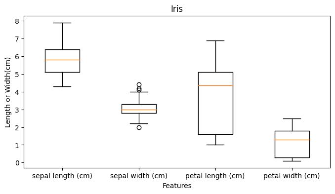
X_df=pd.DataFrame(X)  #boxplot()함수 사용을 위해 데이터 프레임 변환

X_df.columns=iris.feature_names # 특성 이름 열 이름으로 대체

X_df['species']=y

print(X_df)
sepal length (cm) sepal width (cm) petal length (cm) petal width (cm) \
0 5.1 3.5 1.4 0.2
1 4.9 3.0 1.4 0.2
2 4.7 3.2 1.3 0.2
3 4.6 3.1 1.5 0.2
4 5.0 3.6 1.4 0.2
.. ... ... ... ...
145 6.7 3.0 5.2 2.3
146 6.3 2.5 5.0 1.9
147 6.5 3.0 5.2 2.0
148 6.2 3.4 5.4 2.3
149 5.9 3.0 5.1 1.8
species
0 0
1 0
2 0
3 0
4 0
.. ...
145 2
146 2
147 2
148 2
149 2
[150 rows x 5 columns]sns.pairplot(X_df, hue='species', height=2)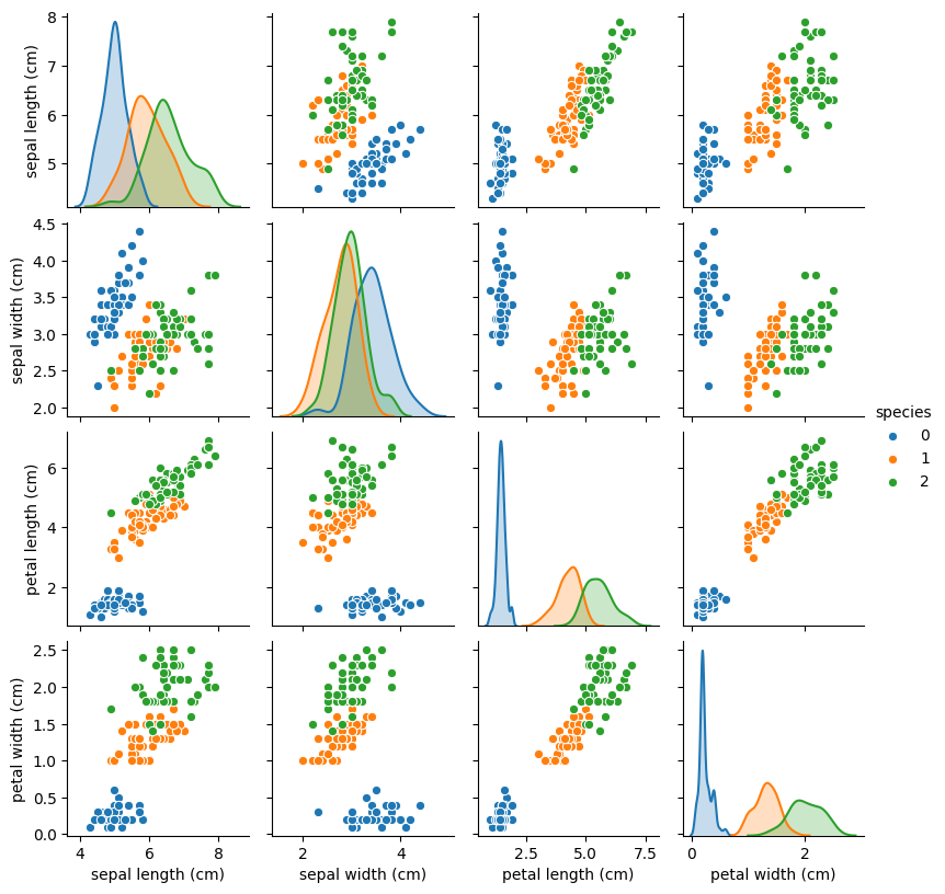
4. 데이터 분리
X_train, X_test, y_train, y_test = train_test_split(X,y,test_size=0.3)5. 피처 스케일링
scalerX=StandardScaler()
scalerX.fit(X_train)
X_train_std=scalerX.transform(X_train)
X_test_std=scalerX.transform(X_test)
6. 모형화 및 학습
model=Perceptron(verbose=1)
model.fit(X_train_std,y_train)
-- Epoch 1
Norm: 3.02, NNZs: 4, Bias: 0.000000, T: 105, Avg. loss: 0.004369
Total training time: 0.00 seconds.
-- Epoch 2
Norm: 3.02, NNZs: 4, Bias: 0.000000, T: 210, Avg. loss: 0.000000
Total training time: 0.00 seconds.
-- Epoch 3
Norm: 3.02, NNZs: 4, Bias: 0.000000, T: 315, Avg. loss: 0.000000
Total training time: 0.00 seconds.
-- Epoch 4
Norm: 3.02, NNZs: 4, Bias: 0.000000, T: 420, Avg. loss: 0.000000
Total training time: 0.00 seconds.
-- Epoch 5
Norm: 3.02, NNZs: 4, Bias: 0.000000, T: 525, Avg. loss: 0.000000
Total training time: 0.00 seconds.
-- Epoch 6
Norm: 3.02, NNZs: 4, Bias: 0.000000, T: 630, Avg. loss: 0.000000
Total training time: 0.00 seconds.
-- Epoch 7
Norm: 3.02, NNZs: 4, Bias: 0.000000, T: 735, Avg. loss: 0.000000
Total training time: 0.00 seconds.
Convergence after 7 epochs took 0.00 seconds
-- Epoch 1
Norm: 1.85, NNZs: 4, Bias: -2.000000, T: 105, Avg. loss: 0.701329
Total training time: 0.00 seconds.
-- Epoch 2
Norm: 3.98, NNZs: 4, Bias: 1.000000, T: 210, Avg. loss: 0.545394
Total training time: 0.00 seconds.
-- Epoch 3
Norm: 4.14, NNZs: 4, Bias: -1.000000, T: 315, Avg. loss: 0.808579
Total training time: 0.00 seconds.
-- Epoch 4
Norm: 5.02, NNZs: 4, Bias: -1.000000, T: 420, Avg. loss: 0.676848
Total training time: 0.00 seconds.
-- Epoch 5
Norm: 6.59, NNZs: 4, Bias: -1.000000, T: 525, Avg. loss: 0.787455
Total training time: 0.00 seconds.
-- Epoch 6
Norm: 5.52, NNZs: 4, Bias: -1.000000, T: 630, Avg. loss: 0.698311
Total training time: 0.00 seconds.
-- Epoch 7
Norm: 5.54, NNZs: 4, Bias: -2.000000, T: 735, Avg. loss: 0.644139
Total training time: 0.00 seconds.
Convergence after 7 epochs took 0.00 seconds
-- Epoch 1
Norm: 3.94, NNZs: 4, Bias: -3.000000, T: 105, Avg. loss: 0.119225
Total training time: 0.00 seconds.
-- Epoch 2
Norm: 4.58, NNZs: 4, Bias: -4.000000, T: 210, Avg. loss: 0.117215
Total training time: 0.00 seconds.
-- Epoch 3
Norm: 5.79, NNZs: 4, Bias: -4.000000, T: 315, Avg. loss: 0.104179
Total training time: 0.00 seconds.
-- Epoch 4
Norm: 5.86, NNZs: 4, Bias: -5.000000, T: 420, Avg. loss: 0.095289
Total training time: 0.00 seconds.
-- Epoch 5
Norm: 7.06, NNZs: 4, Bias: -5.000000, T: 525, Avg. loss: 0.056061
Total training time: 0.00 seconds.
-- Epoch 6
Norm: 7.47, NNZs: 4, Bias: -6.000000, T: 630, Avg. loss: 0.095611
Total training time: 0.00 seconds.
-- Epoch 7
Norm: 7.88, NNZs: 4, Bias: -7.000000, T: 735, Avg. loss: 0.093122
Total training time: 0.00 seconds.
-- Epoch 8
Norm: 7.17, NNZs: 4, Bias: -8.000000, T: 840, Avg. loss: 0.019793
Total training time: 0.00 seconds.
-- Epoch 9
Norm: 9.08, NNZs: 4, Bias: -7.000000, T: 945, Avg. loss: 0.082413
Total training time: 0.00 seconds.
-- Epoch 10
Norm: 8.29, NNZs: 4, Bias: -8.000000, T: 1050, Avg. loss: 0.045435
Total training time: 0.00 seconds.
-- Epoch 11
Norm: 8.41, NNZs: 4, Bias: -8.000000, T: 1155, Avg. loss: 0.067990
Total training time: 0.00 seconds.
-- Epoch 12
Norm: 8.56, NNZs: 4, Bias: -8.000000, T: 1260, Avg. loss: 0.062187
Total training time: 0.00 seconds.
-- Epoch 13
Norm: 7.87, NNZs: 4, Bias: -9.000000, T: 1365, Avg. loss: 0.082040
Total training time: 0.00 seconds.
Convergence after 13 epochs took 0.00 seconds[Parallel(n_jobs=1)]: Using backend SequentialBackend with 1 concurrent workers.
[Parallel(n_jobs=1)]: Done 3 out of 3 | elapsed: 0.0s finishedPerceptron(verbose=1)In a Jupyter environment, please rerun this cell to show the HTML representation or trust the notebook.
On GitHub, the HTML representation is unable to render, please try loading this page with nbviewer.org.
Perceptron(verbose=1)
# 가중치
print(model.coef_)
# 편향
print(model.intercept_)
[[-1.35951428 1.97275265 -1.46733157 -1.0997214 ]
[-0.91929061 -1.69928112 4.06213278 -3.23501377]
[-1.60316749 -0.19414391 5.45511955 5.44362091]]
[ 0. -2. -9.]7. 예측
y_pred=model.predict(X_test_std)print(y_pred) #예측값
print(y_test) #실제값[1 0 2 2 0 0 2 2 0 1 0 2 0 1 2 1 1 2 0 0 0 2 0 0 1 0 2 2 0 0 2 0 0 0 0 0 2
2 2 0 2 0 0 2 2]
[1 1 2 2 1 0 2 2 0 2 1 2 0 1 2 1 1 2 0 0 0 2 0 0 1 1 2 2 0 0 2 0 0 0 1 0 2
2 2 0 2 0 1 2 2]print('Accuracy:%.2f' % accuracy_score(y_test,y_pred))Accuracy:0.84